Perturbative expansions for simulating noisy Clifford circuits

This module enables the simulation of noisy Clifford circuits through a perturbative expansion in the noise parameter (assuming the noise is small). Instead of simulating many Monte Carlo trajectories, only the leading order trajectories are exhaustively enumerated and simulated, supporting even obtaining symbolic expressions for figures of merit.

Purification Circuit Example

Here is an example of a purification circuit (the same circuit seen in the Monte Carlo example)

good_bell_state = S"XX                    ZZ"canonicalize_rref!(good_bell_state)initial_state = MixedDestabilizer(good_bell_state⊗good_bell_state)g1 = sCNOT(1,3) # CNOT between qubit 1 and qubit 3 (both with Alice)g2 = sCNOT(2,4) # CNOT between qubit 2 and qubit 4 (both with Bob)m = BellMeasurement([sMX(3),sMX(4)]) # Bell measurement on qubit 3 and 4v = VerifyOp(good_bell_state,[1,2]) # Verify that qubit 1 and 2 indeed form a good Bell pairepsilon = 0.01 # The error raten = NoiseOpAll(UnbiasedUncorrelatedNoise(epsilon))# This circuit performs a depolarization at rate `epsilon` to all qubits,# then bilater CNOT operations# then a Bell measurement# followed by checking whether the final result indeed corresponds to the correct Bell pair.circuit = [n,g1,g2,m,v]petrajectories(initial_state, circuit)

Dict{CircuitStatus, Float64} with 3 entries:
  failure:CircuitStatus(3)       => 0.0129373
  false_success:CircuitStatus(2) => 0.019406
  true_success:CircuitStatus(1)  => 0.967065

For more examples, see the notebook comparing the Monte Carlo and Perturbative method or this tutorial on entanglement purification.

Symbolic expansions

The perturbative expansion method works with symbolic variables as well. One can use any of the symbolic libraries available in Julia and simply plug symbolic parameters in lieu of numeric parameters. A detailed example is available as a Jupyter notebook.

Interface for custom operations

If you want to create a custom gate type (e.g. calling it Operation), you need to definite the following methods.

applyop_branches!(s::T, g::Operation; max_order=1)::Vector{Tuple{T,Symbol,Real,Int}} where T is a tableaux type like Stabilizer or a Register. The Symbol is the status of the operation, the Real is the probability for that branch, and the Int is the order of that branch.

There is also applynoise_branches! which is convenient for use in NoisyGate, but you can also just make up your own noise operator simply by implementing applyop_branches! for it.

You can also consult the list of implemented operators.

Error Correction in Perturbative Expansion Simulations

Here is an example that demonstrates the simulation of a noisy quantum circuit using perturbative expansions, where error correction is incorporated through a DecoderCorrectionGate. After encoding the Steane code and introducing noise, the decoder correction gate applies the (hopefully) most likely correction based on the measured syndrome, leading to a noticeable improvement in the logical success rate. This illustrates how perturbative expansion methods can be combined with error-correcting circuits to study performance under noise.

Some of the relevant structures and functions used in this code are:

using QuantumCliffordusing QuantumClifford.ECC: Steane7, parity_checks, naive_encoding_circuit, naive_syndrome_circuit, TableDecoder, DecoderCorrectionGate, code_n, code_scode = parity_checks(Steane7()) #creates the stabilizer tableau for the Steane codedata = code_n(code)checks = code_s(code)qbits = data+checksregister = Register(one(MixedDestabilizer, qbits), checks) # A register with 13 qubits, 7 data qubits and 6 ancillasdecoder = TableDecoder(code) # creates a decoder based on the Steane codenoiseless_state = one(MixedDestabilizer, data)encoding_circuit = naive_encoding_circuit(code) # circuit to encode a state in the Steane codespacemctrajectory!(noiseless_state, encoding_circuit) # applies each gate in ecirc to noiseless_stateverify = VerifyOp(noiseless_state, 1:data) # prepare a "tomographic" verification operation, checking that the first 7 qubits of the register indeed form still the same code wordsyndrome_circuit,_,_ = naive_syndrome_circuit(code) # the operations needed to extract the error syndromeepsilon = 0.1noise = NoiseOp(UnbiasedUncorrelatedNoise(epsilon), (1:data)) # an op that introduces noise into the circuitcircuit = vcat(encoding_circuit, noise, syndrome_circuit, verify)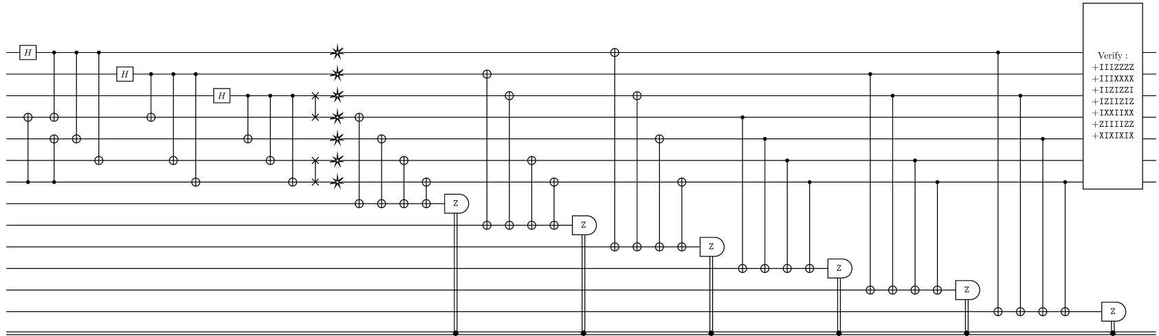

we can run perturbative expansions with petrajectories.

pet = petrajectories(register, circuit; max_order=3)pet

Dict{CircuitStatus, Float64} with 3 entries:
  failure:CircuitStatus(3)       => 0.0
  false_success:CircuitStatus(2) => 0.518805
  true_success:CircuitStatus(1)  => 0.478467

We see that the true_success rate is pretty terrible. In order to improve this rate with the help of error correction, we can use the DecoderCorrectionGate:

correction_gate = DecoderCorrectionGate(decoder, 1:data, 1:checks) # takes in the decoder, data qubits and syndrome bits as an input and guesses the most probable error correcting Pauli Operation based on the recorded syndrome

Let's include the correction gate in our list of circuit operations and place it after syndrome collection.

circuit = vcat(encoding_circuit, noise, syndrome_circuit, correction_gate, verify)pet = petrajectories(register, circuit; max_order=3)pet

Dict{CircuitStatus, Float64} with 3 entries:
  failure:CircuitStatus(3)       => 0.0
  false_success:CircuitStatus(2) => 0.129956
  true_success:CircuitStatus(1)  => 0.867316

We can see that the true_success rate has gone up significantly.